By Ashkan Faghiri Graduate Research Assistant at TReNDS | View Ashkan’s Pubs
Based on an article titled “A unified approach for characterizing static/dynamic connectivity frequency profiles using filter banks“
Filterbanks (a set of filters with different response function operating on the same signal) are useful tools for splitting temporal signals into desired frequency bands. Here we give a very short introduction to a pipeline that uses these frequency decomposition tools for analyzing time-resolved connectivity (also labeled dynamic connectivity and time-varying connectivity). The idea is quite simple and has been published previously [1]. First, a connectivity estimator is used to transform the data from activity space (i.e., fMRI timecourses) to connectivity space (i.e., temporally coherent pairs of fMRI timecourses from voxels, regions, or distributed networks). Second, a filter bank is used to divide the connectivity signals into desired frequency bands. Note, we suggest that the connectivity estimator used in the first step should not perform any filtering in the connectivity space as that filtering would interfere with the filterbank which is used in the second step. There are several estimators that satisfy this requirement: an estimator based on sliding window Pearson correlation (without the last windowing) which is given in equation 1 [1], Instantaneous shared trajectory [IST; 2], elementwise multiplication of temporal derivative [MTD; 3] and even elementwise multiplication of activity time series pairs directly [4].
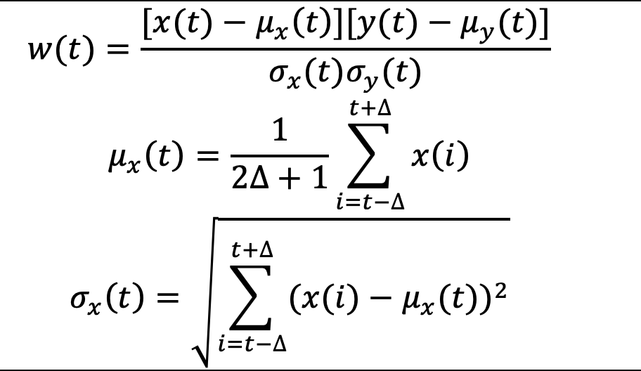
Equation 1

Figure 1: Illustration of filterbank pipeline for time resolved connectivity.
Using filterbanks in this manner provides direct control over the study of connectivity at different frequency bands. Importantly, a method like sliding window Pearson correlation (the most common method to estimate time-resolved connectivity) essentially operates as a lowpass filter in the form of its final sliding window (i.e., moving average operator) but the exact frequency of the estimated connectivity time-series is not immediately clear. Filterbanks essentially require the user to design the filters based on a set of cutoff frequencies for different filters and thus provide additional clarity into the frequency information. Below we share three specific situations where one can design filterbanks in the pipeline based on some assumptions they make:
- Scenario 1: Suppose we do not want to make any assumption about what parts of connectivity bandwidth are “good” so the whole available spectrum is broken into different bands. Additionally, we want to break this signal into 4 bands. The number of bands is a selection that we have to make (similar to how the number of samples in a Fast Fourier transform is selected), based on literature, or based on the specific question we want to answer. The designed filter spectrum is shown in Figure 2.
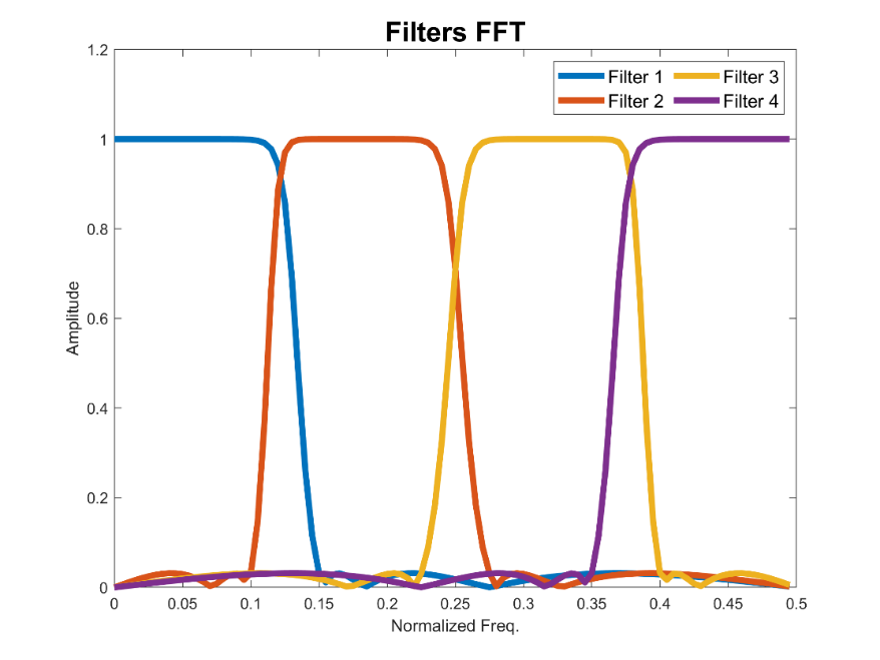
Figure 2: frequency response functions for the four filters defined for scenario 1. As can be seen here all the filters have the same bandwidth.
Now using the pipeline shown in Figure 1, activity time series are transformed into pairwise time-resolved connectivity then passed through all the filters in the filterbank. Figure 3 shows a toy example for this scenario. The left columns show one sample of the activity time-series pair, the middle column shows the true connectivity time series and its estimated value. And the right column shows the true connectivity value for each filter and its estimation.
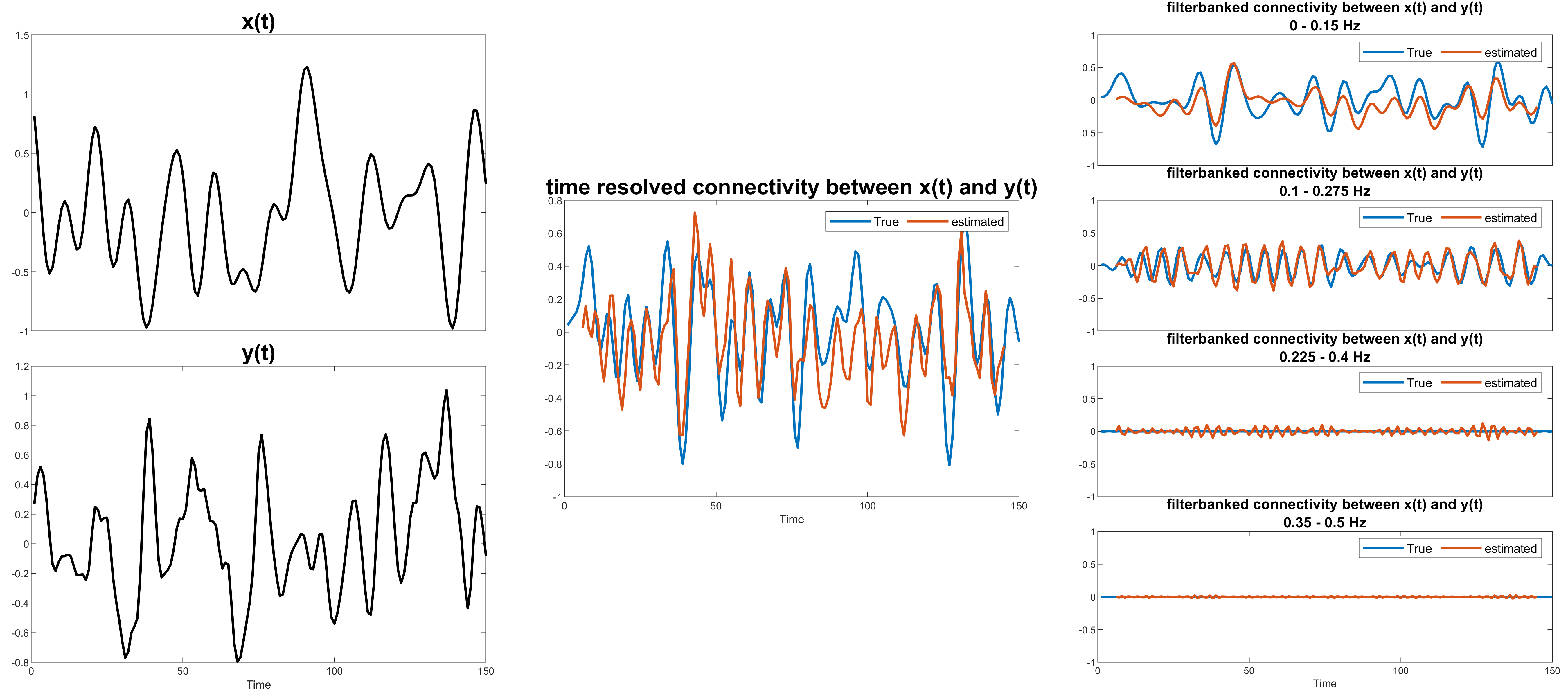
Figure 3: A toy example for scenario 1
- Scenario 2: This scenario is quite similar to the previous one with the difference that we want to design the first filter of the filter bank in such a way that its bandwidth is longer than other filters (see Figure 4).
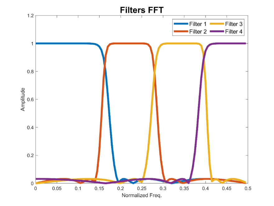
Figure 4: frequency response functions for the four filters defined for scenario 2. As can be seen here the first filter’s bandwidth is larger than other filters’ bandwidth.
Figure 5 shows the toy example for this scenario. Notice how there seems to be more variation in the first filter? This is caused by the choice of larger bandwidth for the first filter made by the user.
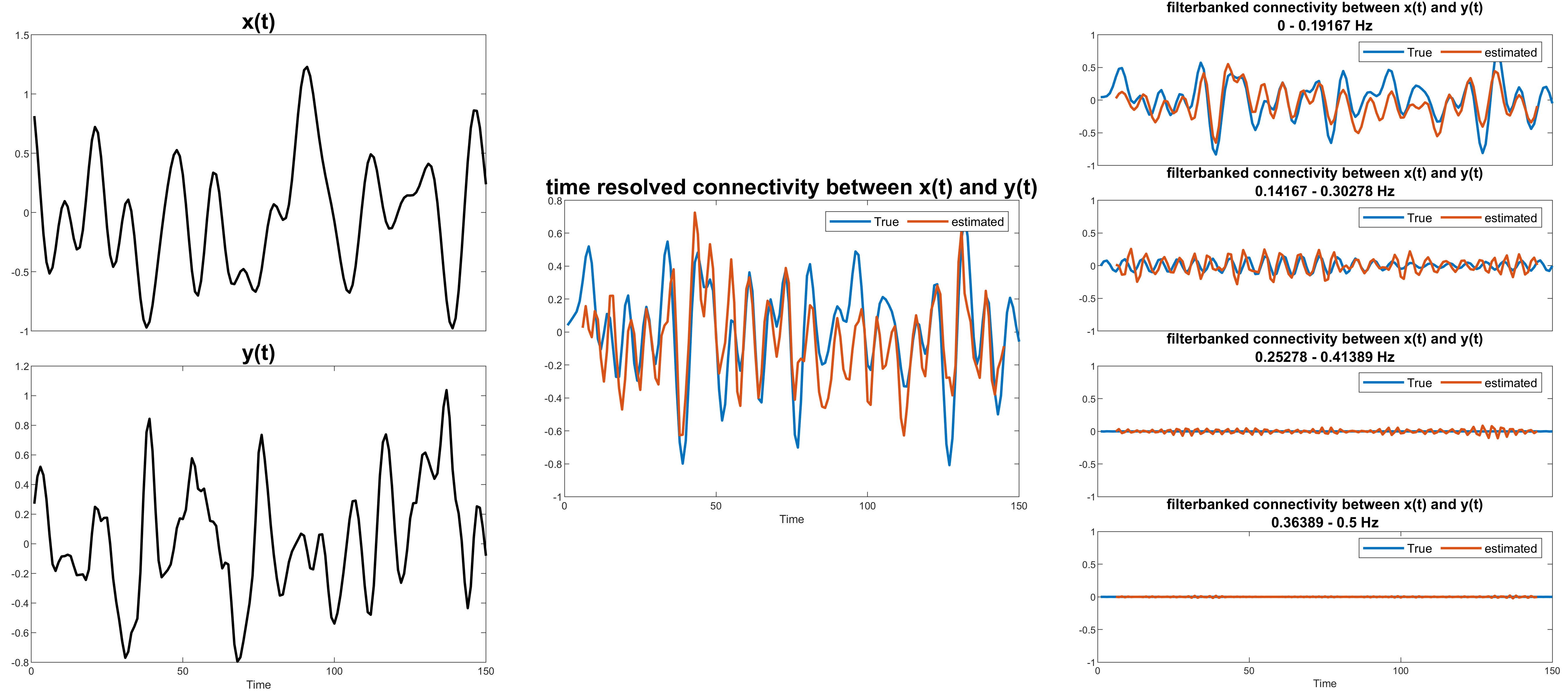
Figure 5: A toy example for scenario 2
- Scenario 3: In this scenario, we assume that a part of the connectivity spectrum is noise, or not of interest, and therefore we choose to remove it (or maybe we want to use the connectivity of that band to provide null or noisy data for statistical inference). Therefore, we design 4 filters with the last high pass filter with a cutoff around 0.2 of normalized frequency to separate undesired values. The frequency response of all 4 filters is shown in Figure 6. The purple line shows the band which is to be removed.
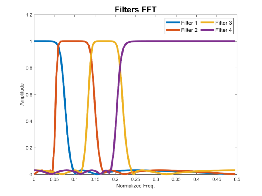
Figure 6: frequency response functions for the four filters defined for scenario 3. As can be seen, the third filter bandwidth is noticeably larger than other filters. This filter output can be used to build a null/noise model for example
Figure 7 shows a toy example for scenario 3 results. Here the estimated connectivity results from the fourth filter are assumed to be noise (based on the assumptions that the user makes). The results from the fourth filter (figure 7 bottom right) can be excluded from further analysis or used as null/noise data for comparison with the signals of interest.
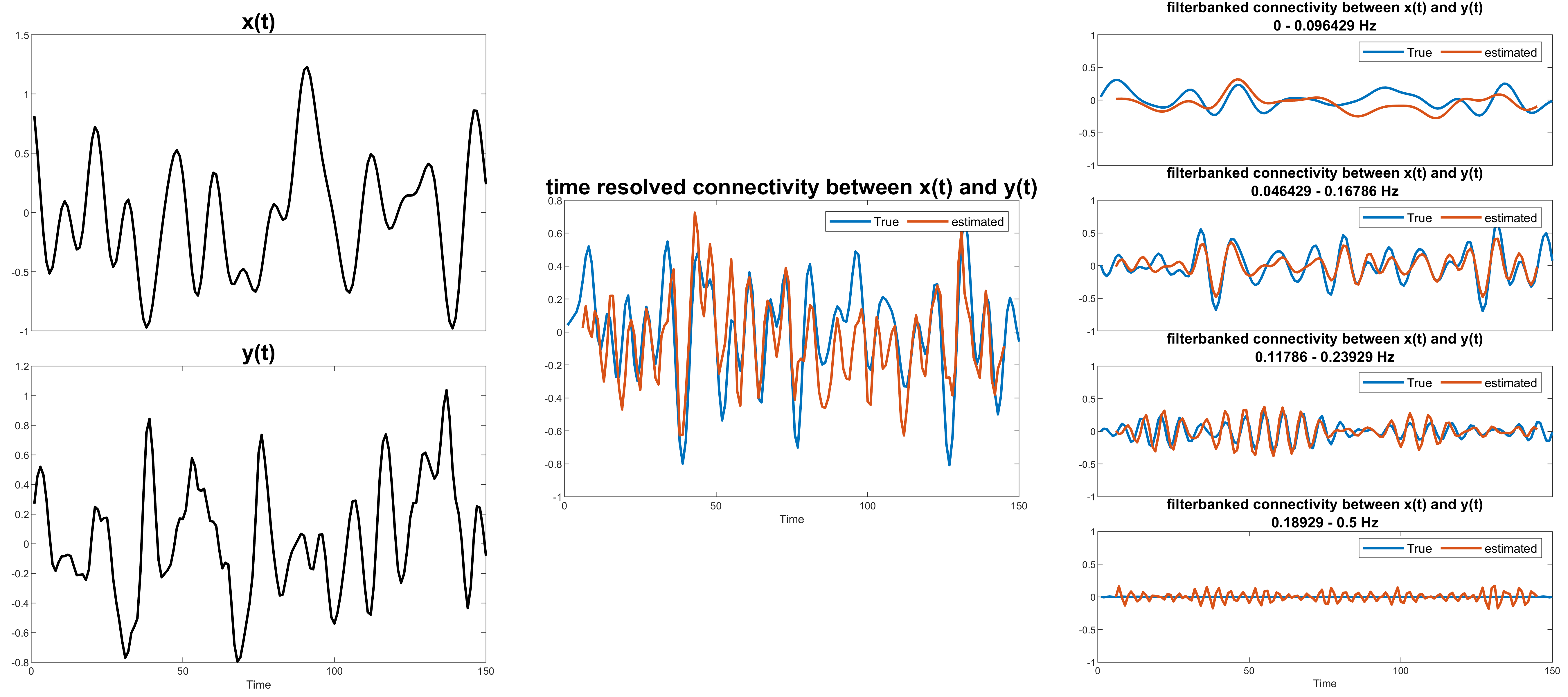
Figure 7: A toy example for scenario 3
Summary: Here, we show how filterbanks can be used in various ways to divide connectivity into different bands of interest or to be used conceptually to generate null results for comparison with the signal of interest. It is important to note that filterbanks have several parameters that needs to be selected. These include filter number, filter type, and filter parameters (like passband ripple, stopband ripple, and transition band length). The number of parameters is relatively small and consistent with other approaches, for example, in sliding window Pearson correlation, one needs to select window size and window shape: these two choices essentially select other filter parameters (a sliding window is literally a lowpass filter). This is also true of many other approaches to time-resolved connectivity which often have implicit parameters that are ‘hidden’. In sum, we believe filter bank connectivity provides a powerful, flexible, and intuitive approach to analysis of time-resolved connectivity.
References:
[1] A. Faghiri, A. Iraji, E. Damaraju, J. Turner, and V. D. Calhoun, “A unified approach for characterizing static/dynamic connectivity frequency profiles using filter banks,” Network Neuroscience, vol. 5, no. 1, pp. 56-82, 2021.
[2] A. Faghiri et al., “Weighted average of shared trajectory: A new estimator for dynamic functional connectivity efficiently estimates both rapid and slow changes over time,” Journal of neuroscience methods, vol. 334, p. 108600, 2020.
[3] J. M. Shine, O. Koyejo, P. T. Bell, K. J. Gorgolewski, M. Gilat, and R. A. Poldrack, “Estimation of dynamic functional connectivity using Multiplication of Temporal Derivatives,” NeuroImage, vol. 122, pp. 399-407, 2015.
[4] J. Faskowitz, F. Z. Esfahlani, Y. Jo, O. Sporns, and R. F. Betzel, “Edge-centric functional network representations of human cerebral cortex reveal overlapping system-level architecture,” Nature neuroscience, vol. 23, no. 12, pp. 1644-1654, 2020.
